Skip to content

Curves & line integrals ​

In this part of the course we work on the following skills:

  • Work with parametric paths
  • Evaluate and work with scalar line integrals
  • Evaluate and work with vector line integrals
  • Work with potentials and conservative vector fields

See also the exercises associated to this part of the course.

Curves have played a part in earlier parts of the course and now we turn our attention to precisely what we mean by this notion. Up until now we relied more on an intuition, an idea of some type of 1D subset of higher dimensional space. We will also define how we can integrate scalar and vector fields along these curves. These types of integrals have a natural and important physical relevance. We will then study some of the properties of these integrals. To start let's recall a random selection of curves we have already seen:

  • Circle: x2+y2=4
  • Semi-circle: x2+y2=4,   x≥0
  • Ellipse: 14x2+19y2=4
  • Line: y=5x+2
  • Line (in 3D): x+2y+3z=0,   x=4y
  • Parabola (in 3D): y=x2,   z=x

In the above list the curves are written in a way where we are describing a set of points using certain constraint or constraints. In some cases in implicit form, in some cases in explicit form. For example, for the circle we formally mean the set {(x,y):x2+y2=4}. We have the idea that the curves should be sets which are single connected pieces and we vaguely have an idea that we need curves that are sufficiently smooth. To proceed we need a precise definition of the 1D objects we can work with. As part of the definition we force a structure which really allows us to work with these objects in a useful way.

Curves, paths & line integrals ​

Let α:[a,b]→Rn be continuous. For convenience, in components we write α(t)=(α1(t),…,αn(t)). We say that α(t) is differentiable if each component αk(t) is differentiable on [a,b] and αk′(t) is continuous

Definition

We say that α(t) is piecewise differentiable if [a,b]=[a,c1]∪[c1,c2]∪⋯∪[cl,b] and α(t) is differentiable on each of these intervals.

Definition

If α:[a,b]→Rn is continuous and piecewise differentiable then we call it a path.

Note that different functions can trace out the same curve in different ways. Also note that a path has an inherent direction. We say that this is a parametric representation of a given curve. We already saw examples of paths in spiral and circular motion. A few examples of paths are as follows.

  • α(t)=(t,t), t∈[0,1]
  • α(t)=(cos⁡t,sin⁡t), t∈[0,2π]
  • α(t)=(cos⁡t,sin⁡t), t∈[−π2,π2]
  • α(t)=(cos⁡t,−sin⁡t), t∈[0,2π]
  • α(t)=(t,t,t), t∈[0,1]
  • α(t)=(cos⁡t,sin⁡t,t), t∈[−10,10]

Observe how some of these paths represent the same curve, perhaps traversed in a different direction.

Let α(t) be a (piecewise differentiable) path on [a,b] and let f:Rn→Rn be a continuous vector field. Recall that we consider α′(t) and f(x) as n-vectors. I.e., in the case n=2, then

α′(t)=(α1′(t)α2′(t)),f(x)=(f1(x)f2(x)).

Definition (line integral of vector field)

Let α(t) be a (piecewise differentiable) path on [a,b] and let f:Rn→Rn be a continuous vector field. The line integral of the vector field f along the path α is defined as

∫f⋅dα=∫abf(α(t))⋅α′(t) dt.

Sometimes the same integral is written as ∫Cf⋅dα to emphasize that the integral is along the curve C. Alternatively the integral is sometimes written as ∫f1 dα1+⋯+fn dαn or ∫f1 dx1+⋯+fn dxn. Each of these different notations are in common usage in different contexts but the underlying quantity is always the same.

Example

Consider the vector field f(x,y)=(y,x3+y) and the path α(t)=(t2,t3) for t∈(0,1). Evaluate ∫f⋅dα.

Solution

We start by calculating

α′(t)=(2t3t2),f(α(t))=(t32t6+t3).

This means that f(α(t))⋅α′(t)=2t52+3t8+3t5 and so

∫f⋅dα=∫01(2t52+3t8+3t5) dt=5942.

Now we consider the question of defining the line integral for scalar fields. Such a line integral allows us also to define the length of a curve in a meaningful way. Again let α(t), t∈[a,b] be a path in Rn and let f:Rn→R be a continuous scalar field.

Definition (line integral of scalar field)

Let α(t), t∈[a,b] be a (piecewise differentiable) path in Rn and let f:Rn→R be a continuous scalar field. The line integral of the scalar field f along the path α is defined as

∫f dα=∫abf(α(t)) ‖α′(t)‖ dt.

Subsequently we will primarily work with the line integral of a vector field. However the analogous results hold also for this integral and the proofs are essentially the same. Namely it is linear and also respects how a path can be decomposed or joined with other paths which changing the value of the integral. Moreover, the value of the integral along a given path is independent of the choice of parametrization of the curve. In this case, even if the curve is parametrized in the opposite direction then the integral takes the same value. Consequently it makes sense to define the length of the curve as the line integral of the unit scalar field, i.e., the length of a curve parametrized by the path α is ∫ab‖α′(t)‖ dt.

Basic properties of the line integral ​

Having defined the line integral, the next step is to clarify its behaviour, in particular the following key properties.

Theorem

Linearity: Suppose f, g are vector fields and α(t) is a path. For any c,d∈R, then

∫(cf+dg)⋅dα=c∫f⋅dα+d∫g⋅dα.

Joining / splitting paths: Suppose f is a vector field and that

α(t)={α1(t)t∈[a,c]α2(t)t∈[c,b]

is a path. Then

∫f⋅dα=∫f⋅dα1+∫f⋅dα2.

Alternatively, if we write C, C1, C2 for the corresponding curves, then

∫Cf⋅dα=∫C1f⋅dα+∫C2f⋅dα.

As already mentioned, for a given curve there are many different choices of parametrization. For example, consider the curve C={(x,y):x2+y2=1,y≥0}. This is a semi-circle and two possible parametrizations are α(t)=(−t,1−t2), t∈[−1,1] and β(t)=(cos⁡t,sin⁡t), t∈[0,π]. These are just two possibilities among many possible choices. For a given curve, to what extent does the line integral depend on the choice of parametrization?

Definition (equivalent paths)

We say that two paths α(t) and β(t) are equivalent if there exists a differentiable function u:[c,d]→[a,b] such that α(u(t))=β(t).

Furthermore, we say that α(t) and β(t) are

  • in the same direction if u(c)=a and u(d)=b,

  • in the opposite direction if u(c)=b and u(d)=a.

With this terminology we can precisely describe the dependence of the integral on the choice of parametrization.

Theorem

Let f be a continuous vector field and let α, β be equivalent paths. Then

∫f⋅dα={∫f⋅dβif the paths in the same direction,−∫f⋅dβif the paths in the opposite direction.

Proof

Suppose that the paths are continuously differentiable path, decomposing if required. Since α(u(t))=β(t) the chain rule implies that β′(t)=α′(u(t)) u′(t). In particular

∫f⋅dβ=∫cdf(β(t))⋅β′(t) dt=∫cdf(α(u(t)))⋅α′(u(t)) u′(t) dt.

Changing variables, adding a minus sign if path is opposite direction because we need to swap the limits of integration, completes the proof.

Gradients & work ​

Let h(x,y) be a scalar field in R2 and recall that the gradient ∇h(x,y) is a vector field. Let α(t), t∈[0,1] be a path. Now let g(t)=h(α(t)), consider the derivative g′(t)=∇h(α(t))⋅α′(t) and evaluate the line integral

∫∇h⋅dα=∫01∇h(α(t))⋅α′(t) dt=∫01g(t) dt=g(1)−g(0)=h(α(1))−h(α(0)).

This equality has the following intuitive interpretation if we suppose for a moment that h denotes altitude. In this case the line integral is the sum of all the infinitesimal altitude changes and equals the total change in altitude.

As a first example of work in physics let's consider gravity. The gravitational field on earth is f(x,y,z)=(00mg). If we move a particle from a=(a1,a2,a3) to b=(b1,b2,b3) along the path α(t), t∈[0,1] then the work done is defined as ∫f⋅dα. We calculate that

∫f⋅dα=∫01f(α(t))⋅α′(t) dt=∫01mg α3′(t) dt=mg [α3(t)]01=mg(b3−a3).

This coincides we what we know, work done depends only on the change in height.

As a second example of work in physics let's consider a particle moving in a force field. Let f be the force field and let x(t) be the position at time t of a particle moving in the field. Let v(t)=x′(t) be the velocity at time t of the particle and define kinetic energy as m2‖v(t)‖2. According to Newton's law f(x(t))=mx″(t)=mv′(t) and so the work done is

∫f⋅dx=∫01f(x(t))⋅v(t) dt=∫01mv′(t)⋅v(t) dt=∫01ddt(m2‖v(t)‖2)=(m2‖v(1)‖2−m2‖v(0)‖2)

In this case we see, as expected, the work done on the particle moving in the force field is equal to the change in kinetic energy.

The second fundamental theorem ​

Recall that, if φ:R→R is differentiable then ∫abφ′(t) dt=φ(b)−φ(a). This is called the second fundamental theorem of calculus and is one of the ways in which we see that differentiation and integration are opposites. The analog for line integrals is the following.

Theorem (second fundamental theorem for line integrals)

Suppose that φ is a continuously differentiable scalar field on S⊂Rn and suppose that α(t), t∈[a,b] is a path in S. Let a=α(a), b=α(b). Then

∫∇φ⋅dα=φ(b)−φ(a).

Proof

Suppose that α(t) is differentiable. By the chain rule ddtφ(α(t))=∇φ(α(t))⋅α′(t). Consequently

∫∇φ⋅dα=∫01∇φ(α(t))⋅α′(t) dt=∫01ddtφ(α(t)) dt.

By the 2nd fundamental theorem in R we know that ∫01ddtφ(α(t)) dt=φ(α(b))−φ(α(a)).

Our earth has mass M with centre at (0,0,0). Suppose that there is a small particle close to earth which has mass m. The force field of gravitation and potential energy are, respectively,

f(x)=−GmM‖x‖3x,φ(x)=GmM‖x‖.

We can calculate ∇φ(x) and see that it is equal to f(x).

The first fundamental theorem ​

First we need to consider a basic topological property of sets. In particular we want to avoid the possibility of the set being several disconnected pieces, in other words we want to guarantee that we can get from one point to another in the set in a way without every leaving the set (see figure).

Definition

The set S⊂Rn is said to be connected if, for every pair of points a,b∈S, there exists a path α(t),t∈[a,b] such that

  • α(t)∈S for every t∈[a,b],
  • α(a)=a and α(b)=b.

Sometimes this property is called "path connected" to distinguish between different notions.
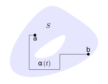
A connected set
A connected set

Recall that, if f:R→R is continuous and we let φ(x)=∫axf(t) dt then φ′(x)=f(x). This is called the first fundamental theorem of calculus and is the other way in which we see that differentiation and integration are opposites. Again we have an analog for the line integral but here it becomes a little more subtle since there are many different paths along which we can integrate between any two points.

Theorem (first fundamental theorem for line integrals)

Let f be a continuous vector field on a connected set S⊂Rn. Suppose that, for x,a∈S, the line integral ∫f⋅dα is equal for every path α such that α(a)=a, α(b)=x. Fix a∈S and define φ(x)=∫f⋅dα. Then φ is continuously differentiable and ∇φ=f.

Proof

As before let e1=(100), e2=(010), e3=(001). Observe that, if we define the paths βk(t)=x+tek, t∈[0,h], then

φ(x+hek)−φ(x)=∫f⋅dβk.

Moreover βk′(t)=ek. Consequently

∂φ∂xk(x)=limh→01h(φ(x+hek)−φ(x))=limh→01h∫0hf(βk(t))⋅ek dt=fk(x).

In other words, we have shown that ∇φ(x)=f(x).

We say a path α(t), t∈[a,b] is closed if α(a)=α(b).

Observe that, if α(t), t∈[a,b] is a closed path then we can divided it into two paths: Let c∈[a,b] and consider the two paths α(t), t∈[a,c] and α(t), t∈[c,b]. On the other hand, suppose α(t), t∈[a,b] and β(t), t∈[c,d] are two path starting at a and finishing at b. The these can be combined to define a closed path (by following one backward).

Definition (conservative vector field)

A vector field f, continuous on S⊂Rn is conservative if there exists a scalar field φ such that, on S,

f=∇φ.

Note that some authors call such a vector field a gradient (i.e., the vector field is the gradient of some scalar). If f=∇φ then the scalar field φ is called the potential (associated to f). Observe that that the potential is not unique, ∇φ=∇(φ+C) for any constant C∈R.

Theorem (conservative fields)

Let S⊂Rn and and consider the vector field f:S→Rn. The following are equivalent:

  1. f is conservative, i.e., f=∇φ on S for some φ,
  2. ∫f⋅dα does not depend on α, as long as α(a)=a, α(b)=b,
  3. ∫f⋅dα=0 for any closed path α contained in S.

Proof

In the previous theorems (the two fundamental theorems) we proved that (i) is equivalent to (ii).

Now we prove that (ii) implies (iii): Let α(t) be a closed path and let β(t) be the same path in the opposite direction. Observe that ∫f⋅dα=−∫f⋅dβ but that ∫f⋅dα=∫f⋅dβ and so ∫f⋅dα=0.

It remains to prove that (iii) implies (ii): The two paths between a and b can be combined (with a minus sign) to give a closed path.

Theorem (mixed partial derivatives)

Suppose that S⊂R2 and that f:S→R2 is a differentiable vector field and write f=(f1f2).

If f is conservative then, on S,

∂f1∂y=∂f2∂x.

The above result is a special case of the following general statement which holds in any dimension.

Theorem (mixed partial derivatives)

Suppose that f is a differentiable vector field[^1] on S⊂Rn. If f is conservative then, for each l,k,

∂fl∂xk=∂fk∂xl.

Proof

By assumption the second order partial derivatives exist and so

∂fl∂xk=∂2φ∂xk∂xl=∂2φ∂xl∂xk=∂fk∂xl.

Example

Consider the vector field

f(x,y)=(−y(x2+y2)−1x(x2+y2)−1)

on S=R2∖(0,0). Calculating we verify that ∂f1∂y=∂f2∂x on S. We now evaluate the line integral ∫f⋅dα where α(t)=(acos⁡t,asin⁡t), t∈[0,2π]. We calculate that

α′(t)=(−asin⁡tacos⁡t),f(α(t))=1a2(−asin⁡tacos⁡t).

This means that

∫f⋅dα=∫02π(sin2⁡t+cos2⁡t) dt=2π.

Observe that in the above example S is somehow not a "nice" set because of the "hole" in the middle. Moreover, observe that the line integral is the same for any circle, independent of the radius.

The mixed partials theorem isn't useful in showing that a vector field is conservative because it is possible for the mixed partial derivatives to all be equal but still the field fail to be conservative. On the other hand, if a pair of mixed derivatives is not equal then f is not conservative and so it is useful for proving the negative. Later in this chapter we will return to this topic.

Potentials & conservative vector fields ​

We now turn our attention to the following question: Suppose we are given a vector field f and we know that f=∇φ for some φ. How can we find φ? For this we consider two methods in the following paragraphs.
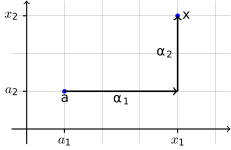
Graph of two straight paths
The paths α1 and α2.

First we describe the method which we call constructing a potential by line integral. Suppose that f is a conservative vector field on the rectangle [a1,b1]×[a2,b2]. We define φ(x) as the line integral ∫f⋅dα where α is a path between a=(a1,a2) and x. For any x=(x1,x2)∈R2 consider the two paths:

  • α1(t)=(t,a2), t∈[a1,x1],

  • α2(t)=(x1,t), t∈[a2,x2].

Let α(t) denote the concatenation of the two paths. We calculate that

∫f⋅dα=∫a1x1f(α1(t))⋅α1′(t) dt+∫a2x2f(α2(t))⋅α2′(t) dt.

This means that φ(x)=∫a1x1f1(t,a2) dt+∫a2x2f2(x1,t) dt.

Now we describe a different method which we describe as constructing a potential by indefinite integrals. Again suppose that f=∇φ for some scalar field φ(x,y) which we wish to find. Observe that ∂φ∂x=f1 and ∂φ∂y=f2. This means that

∫axf1(t,y) dt+A(y)=φ(x,y)=∫byf2(x,t) dt+B(x)

where A(y), B(x) are constants of integration. Calculating and comparing we can then obtain a formula for φ(x,y).

Find a potential for f(x,y)=(exy2+12exy) on R2.

We calculate that

∫axf1(t,y) dt+A(y)= exy2+x+A(y)=φ(x,y),∫byf2(x,t) dt+B(x)=exy2+B(x)=φ(x,y).

From this we see that we can choose A(y)=0 and B(x)=x to obtain equality of the above quantities. Consequently we obtain the potential φ(x,y)=exy2+x.

The mixed partials theorem concerning conservative fields and the mixed partial derivatives was somewhat less than satisfactory since the converse wasn't possible. In order to get a more satisfactory result we need to look at another topological details of the domain of the vector field. This concept is somewhat suggested by the methods of constructing potentials which were described above.

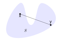
Definition (convex)

A set S⊂Rn is said to be convex if for any x,y∈S the segment {tx+(1−t)y,t∈[0,1]} is contained in S.
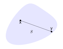
A convex set
A convex set
A set which is not convex
A set which is not convex.

This extra property permits the following sufficient condition for a vector field to be conservative.

Theorem

Let f be a differentiable vector field on a convex region S⊂Rn. Then f is conservative if and only if

∂fl∂xk=∂fk∂xl,for each l,k.

Proof

We have already proved that f being conservative implies the equality of partial derivatives (mixed partials theorem) and therefore we need only assume that ∂gfl=∂lfk and construct a potential. Let φ(x)=∫f⋅dα where α(t)=tx, t∈[0,1]. Since α′(t)=x, φ(x)=∫01f(tx)⋅x dt. Also (needs proving)

∂φ∂xk(tx)=∫01(t∂kf(tx)⋅x+fk(tx)) dt.

This is equal to ∫01(t∇fk(tx)⋅x+fk(tx)) dt because ∂gfl=∂lfk; By the chain rule applied to g(t)=t∇fk(tx) this is equal to fk(x) as required.

The above gives us a useful tool to check if a given vector field is conservative. Using the idea of "gluing together" several convex regions this result can be manually extended to some more general settings. Later, we will take advantage of some further ideas in order to significantly extend this result.